14 June, 2026

Also available as a slide deck.

Issues: 1) The hamiltonian I used and the one of Hénon-Heiles, I oversaw a prefactor of \(1/2\)

\[U(x,y)= \frac{m\omega^2}{2}(x^2+y^2)+\alpha(x^2y-\frac{y^3}{3}).\]

The potential used by Hénon and Heiles (1964)

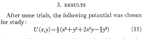
which translates to \(\alpha=1.0\), \(m=1\) and \(\omega=1\).

This results in the following plots depict the difference

\(\alpha=1\)

\(\alpha=2\)

The specific detail I obtain from this plot is, the initial-conditions-space that I need to sample.

• I need to sample:

1. (\(x\), \(y\))–plane
2. (\(p_x\), \(p_y\))–plane
3. even distribution,
4. weighted distribution based on regions of interest, i.e a “zoom”

• I need to estimate the time of these simulations
• I need to understand the analysis too of my cut through the phase plane, i.e. why do I not see it below in the appropriate plots

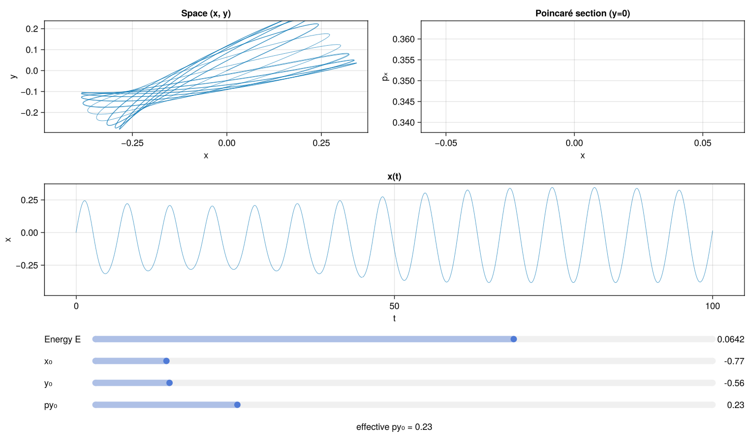
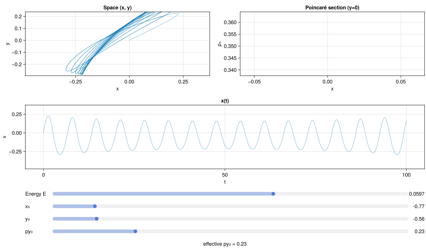
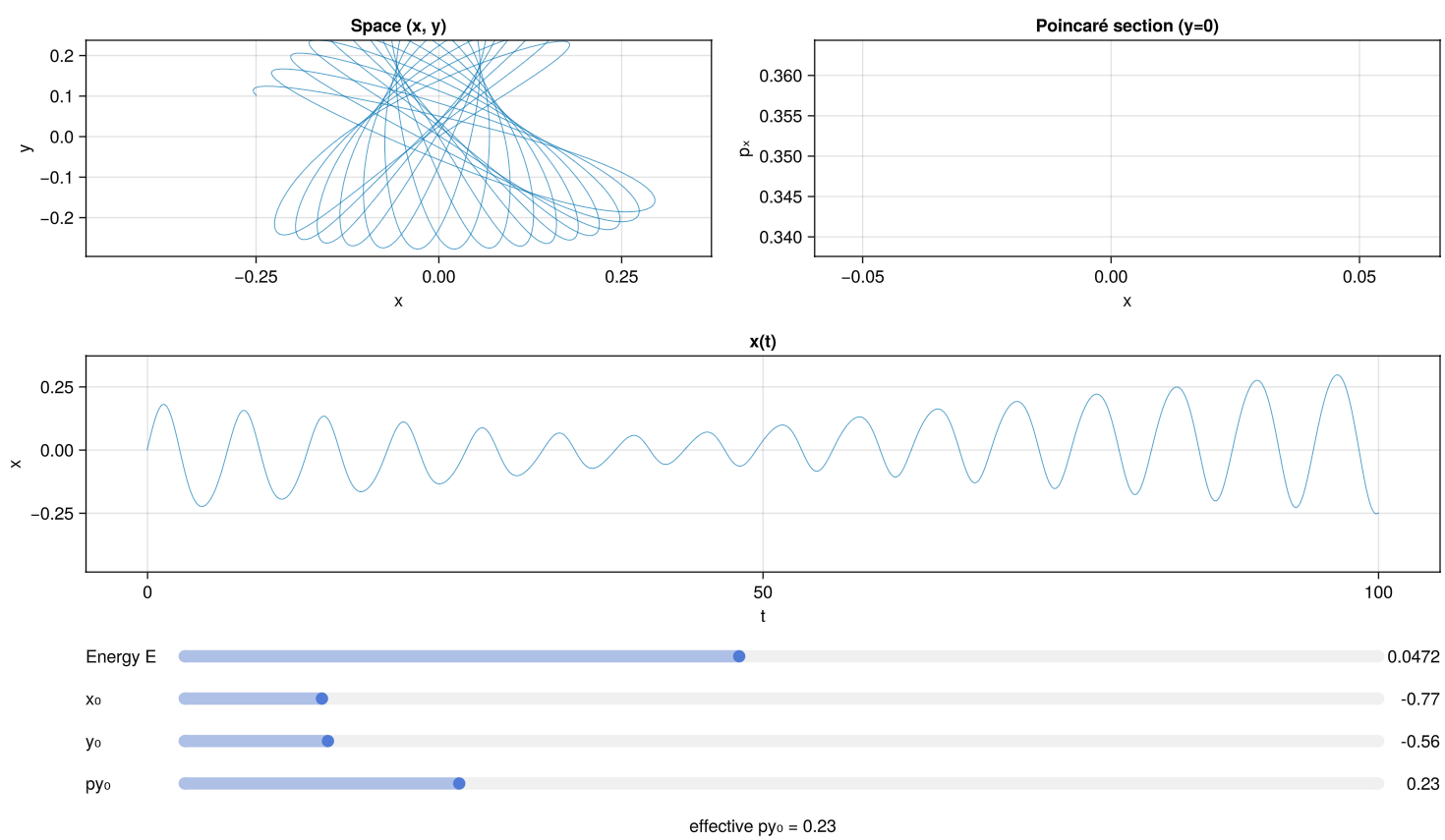
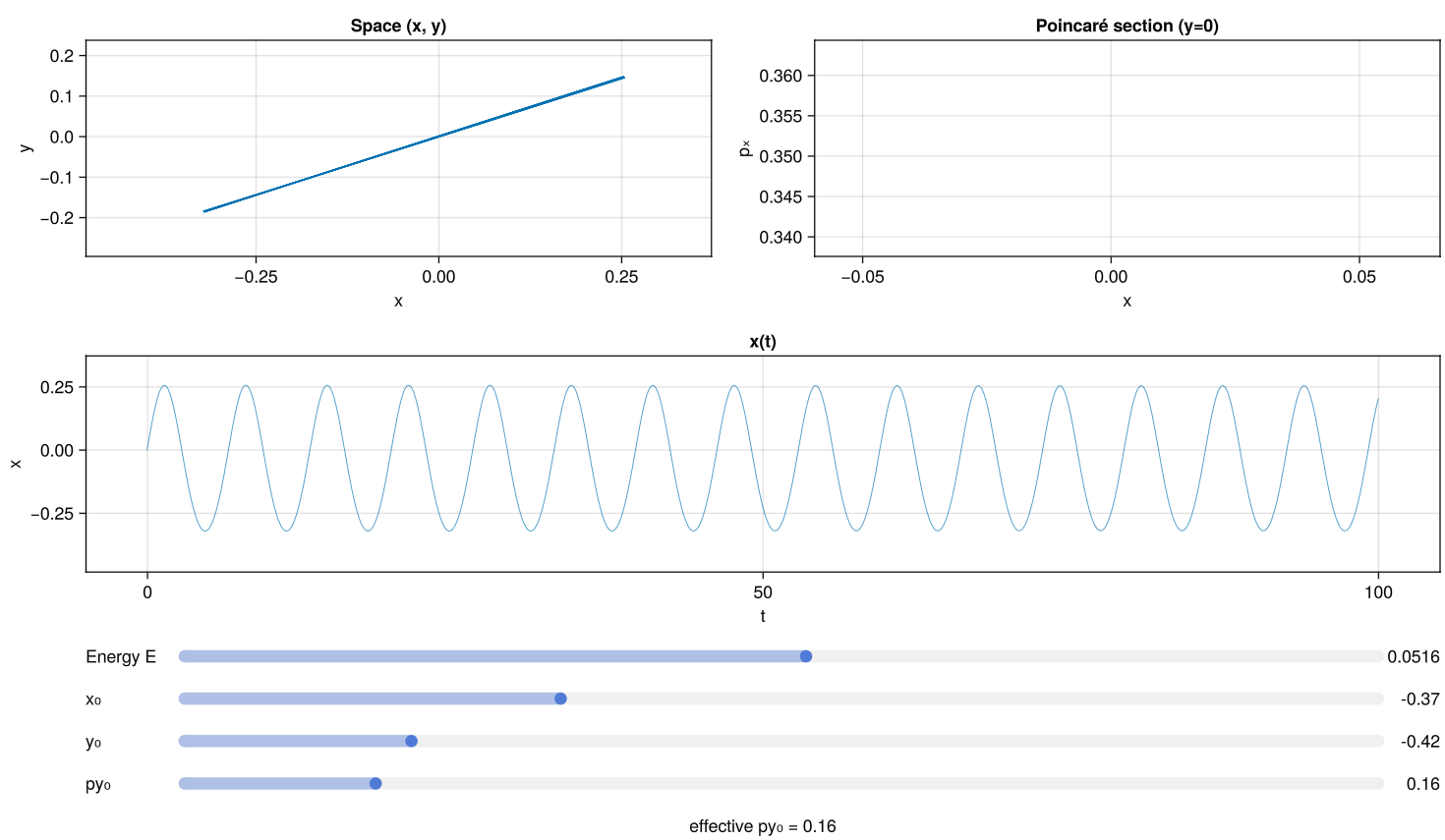
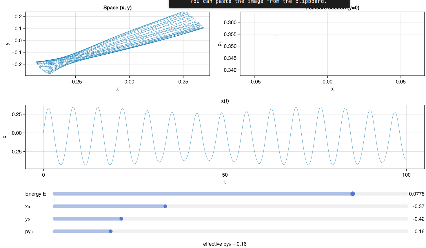
I have made the following observations running the following interesting observations of transitions, sudden changes on the kind of trajectories made in the x-y plane

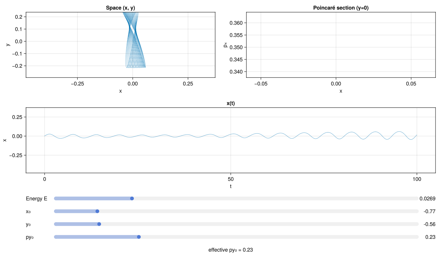
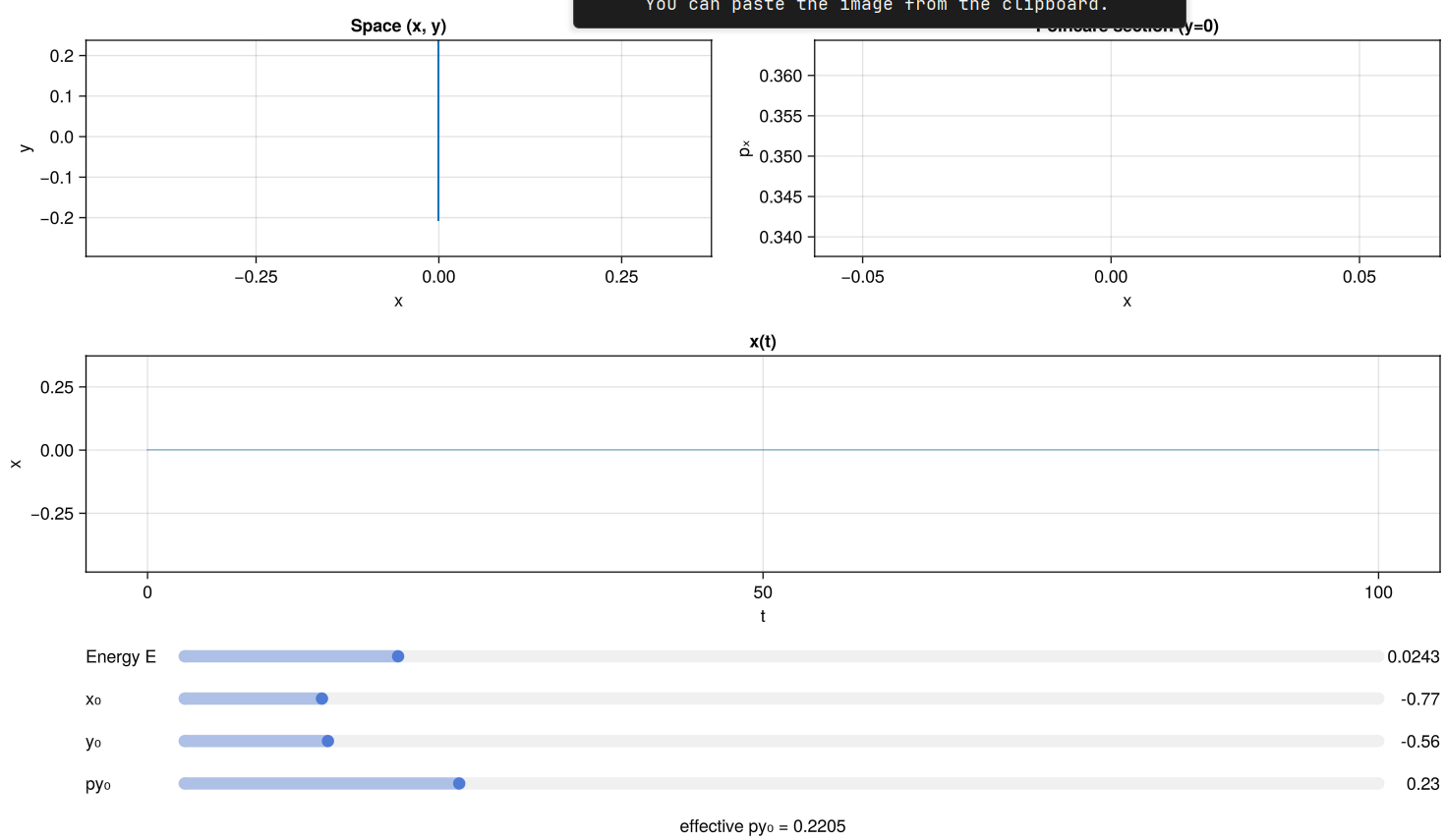
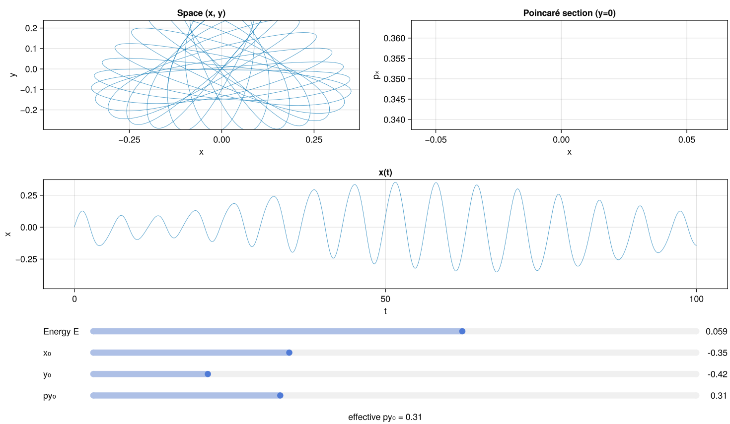
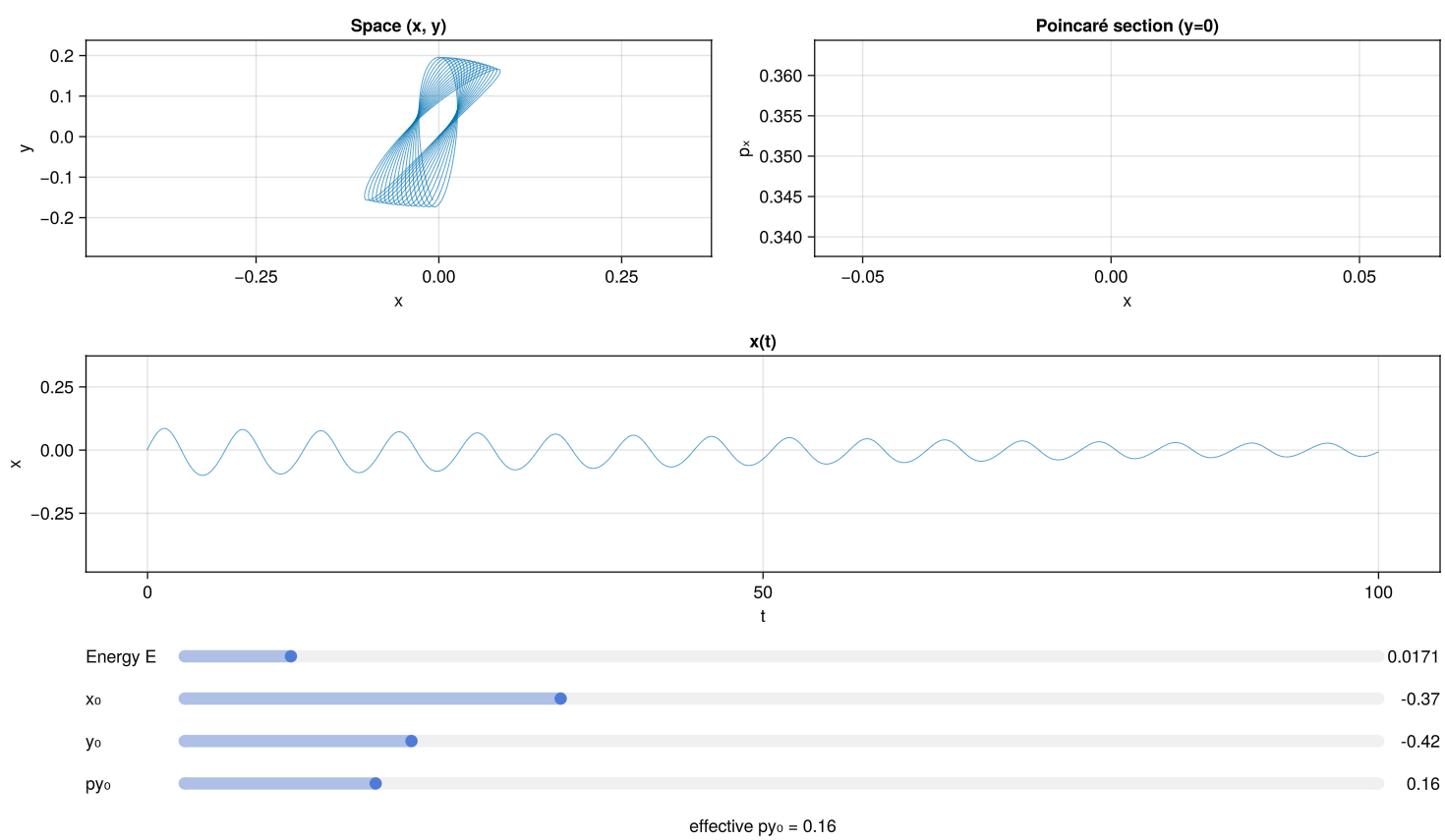
References

Hénon, Michel, and Carl Heiles. 1964. “The Applicability of the Third Integral of Motion: Some Numerical Experiments.” The Astronomical Journal 69 (1): 73–79. https://doi.org/10.1086/109234.