Day Logs
To do!
- So now that I have a general idea, how the phase space is changing in between \(E \in (-0.5, -0.3)\) I am now curious to see how the indiviual trajectories for the interesting periodic orbits behave
-
naming of periodic orbits
So I am currently studying two specific periodic orbits. I call these orbit ‘A’. There is one which is there from \(E = -\infty\) and has a period of \(p=1\), in the sense of poincaré maps, \(M:\Sigma -> \Sigma\). Hence the name of that orbit \(A1\).
Then there is a periodic orbit, with period \(p=3\). Its origin is yet unknown, but seems to come into existance, due to the ‘detection’ of one outer wall.
Lost Wonderers Thoughts:
To do!
tracing surface of section
I have two scans where I search periodic orbits and look random trajectories, in order to see how the structures change for the various energy shells between \(E_1=-0.5\) and \(E_2=-0.3\). This region is particular interesting, as this region is where the structure of phasespac change from partially structured system to a completly chaotic system.


A particular interesting region, is the energy range: \(E=-0.45765\frac{\mathcal{C}}{L}\) and \(E=-0.43882 \frac{\mathcal{C}}{L}\).


I also tested this transition for various gap sizes, though the simulation for \(del=10^{-3}, 10^{-5}, 10^{-8}\) still crashes for the chaotic region. Interestingly the qualitatively, the region inspected (\(E\in[-0.5,-0.3]\)) seems qualitatively unaffected.
Here is one energy picked randomly, to allow for a comparison.
E=-0.391 C/L


Lost Wonderers Thoughts:
To do!
Unordered notes
So I am starting to further the the study of change of the topology and geometry of the attractive case of the model, I will describe this in ‘Renormalisation’
- I need to think about the time units
Renormalisation
So I am considering the case that the displayed, relative volume should be a constant value \(c\). I am looking for \(\epsilon\), to find how the width should be displayed.
\[\frac{\int_{-\epsilon}^{\epsilon} x(p)dp}{\int_{-\infty}^{\infty} x(p)dp}=c\]
The Lorenzian function \(x(p)\propto \tfrac{1}{2m_2E-p^2}\) is obtained by Looking at the boundary of the surface of section. If the boundary is considered, we obtain
\[x(p)= \frac{2m_2 \mathcal{C}}{L} \frac{1}{2m_2E-p^2}-\partial\mathcal{B}_{1\text{R}}\]
The integral of the lorenzian term is
\[\int_{-\infty}^{\infty}\frac{dp}{p^2+\kappa^2} = \frac{\pi}{\kappa}, \qquad \int_{-\varepsilon}^{\varepsilon}\frac{dp}{p^2+\kappa^2} = \frac{2}{\kappa}\arctan\frac{\varepsilon}{\kappa}\] \[\frac{2}{\pi}\arctan\frac{\varepsilon}{\kappa} = c \quad\Longrightarrow\quad \boxed{\varepsilon = \sqrt{-2mE}\;\tan\!\left(\frac{\pi c}{2}\right)}, \qquad 0<c<1.\]
As the boundary only funcitons as an offset, and only cases \(E<0\) shall be considered, this consideres the problem to be solved.
Lost Wonderers Thoughts:
When discussing with Awais, he suggested, attractive and repulsive should behave the same, with the difference of changing the order of the boxes?
To do!
quesitons
- Why do I considere lyapunov exponents near the periodic orbits?
- linearizaiton only makes sense near the periodic orbits?
The effect of the distance
It seems as if the distance between the boxes has a qualitative effect on the dynamics only after DEL>1e-6. Thus for now, I will choose DEL=1e-8 as the distance between the boxes. And later investigate the effect on the dynamics of the distance between the boxes again.
.png)
.png)
.png)
.png)
.png)
.png)
Lost Wonderers Thoughts:
I watched a lecture by Tim Palmers interpretation on quantum mechanics, i.e. the Bell inequality. He calls invariant set theory.
Here the idea is that the underlying assumptions about the Bell’s inequality are not in line with reality, that state space is a smooth and continuous state space, but is rather fractal, thus determanistically indeterminable. The experimental assumptions, that each photon is the same, cannot be fulfilled; each photon originates from a different location in phase space, and thus the assumption, that the photons are locally the same are broken.
::: ::: {.callout-note collapse=“true”} ## 21 September, 2026
To do!
Units of my system
My hamiltoninan \(H(u)=H(x_1,x_2,p_1,p_2)\) is given by the electromagnetic interaction potential \(V(x_1,x_2)\), and the reflecting boundaries potnetial \(V_b\), and of course the kinetic terms \(T(p_i)\)
\[H(u)=\frac{p_1^2}{2m_1}+\frac{p_2^2}{2m_2}+\frac{\mathcal{C}}{|x_1-x_2|}+V_b(x_1)+V_b(x_2)\]
Where as \(V_b(x_i)\) is to be understood as a refelecting boundary \(\partial \mathcal{B}\) that traps particle \(i\), so \(x_i\in\mathcal{B}\). So when \(x_i\) crosses the boundary the conjugate momentum is inverted \(p_i \to -p_i\). Motivated by thermodynamical settings, in which two isolated systems exchange heat, we considere a partition on \(\mathcal{B}=\mathcal{B}(1) \cup \mathcal{B}(2)\), with no overlap \(\mathcal{B}(1)\cap \mathcal{B}(2)=\emptyset\). We define the boundary in coordinates by an open interval \(\mathcal{B}(i)=(b_i-L,b_i+L)\), with boundaries at \(\partial\mathcal{B}=b_i\pm L\). The partition is created by choosing \(b_1 < b_2\) sattisfying \(b_1+L < b_2-L\). A result of the partitioning is a serperation distance \(\delta = b_1+L- (b_2-L)=b_1-b_2+2>0\).
The boundary potential can then be defined as \[V_b(x_i) =\Bigg\{\begin{matrix} 0 & \text{ if } x_i \in \mathcal{B}(i),\\ \infty & \text{ if } x_i \not\in \mathcal{B}(i). \end{matrix} \]
The hamiltonian for inside the boundary \(x_1,x_2 \in \mathcal{B}\), then becomes \[H(u)=\frac{p_1^2}{2m_1}+\frac{p_2^2}{2m_2}+\frac{C}{|x_1-x_2|}\]
I want to investigate the characteristic units of my system. As my boundary defines a characteristic length scale \(L\), to which the particle positions are confind to. I will write the units of the dimesion in brackets, i.e. meters \([\text{m}]\)
\[ \begin{align} x [\text{m}] \to \hat{x}[\text{L}]&=\tfrac{x}{L} [\text{L}] \\ \Leftrightarrow x [\text{m}] &= L\hat{x} \end{align} \]
How did this effect my Hamiltonina \(H\)? The interaction term gets transformed: \[V(x_1-x_2)= \frac{\mathcal{C}}{|x_1-x_2|}= \frac{\mathcal{C}/L}{|\hat{x}_1-\hat{x}_2|}\]
This results in a natural units of energy to be given by the relation of the characteristic interaction strength \(\mathcal{C}\) per characteristic length scale \(L\). So we considere in relation to the \(\mathcal{C}/L\): \[\frac{H(u)}{\mathcal{C}/L} = \frac{p_1^2}{2m_1\,\mathcal{C}/L}+\frac{p_2^2}{2m_2\,\mathcal{C}/L}+\frac{1}{|\hat{x}_1-\hat{x}_2|}=\frac{E}{\mathcal{C}/L}.\]
With the dimensions of energy given by \(\mathcal{C}/L\).
How about the units of momentum and time? Energy is in units \(E_{\text{sys}}[\mathcal{C}/L]\) and in units of length \(L\), mass \(\text{}\) and time \(\text{t}\), \(E_{\text{SI}}[(L/\text{t})^2\text{m}]\) we can equate these \(E_{\text{sys}}=E_{\text{SI}}\) to obtain the units of time:
\[\begin{align} 1[(L/\text{t})^2\text{m}]&=1[\mathcal{C}/L]\\ 1[\text{t}^2] &=1[L^3\text{m}/\mathcal{C}] \end{align}\]
Here a suggestion, without much thought: As a simple model, I will set \(m_1=m_2=1\text{m}\) so that both point mass are the same, and would simplify my units for the system.
surface of section
Yet again, considering the boundary of the surface of section: The surface of section will be a plane which position depends on the sign of the characteristic interaction strenght \(\mathcal{C}\). If \(\mathcal{C}<0\) then the ineraction is repulsive and the boundaries further apart, are sure to make contact, where as the opposite is the case for \(\mathcal{C}>0\). Thus, without loss of generality, we choose particle \(1\) as the conditional particle. Depending on the sign of the characteristic interaction strenght \(\mathcal{C}\) either \(\partial \mathcal{B}(1,1)\) (\(\mathcal{C}<0\), repulsive) or \(\partial \mathcal{B}(1,2)\) (\(\mathcal{C}>0\), attractive) will mark the point that span the surface of section \(\Sigma=\text{span}(x_2,p_2)\). We shall refere to the boundary of particle \(1\) as \(\partial \mathcal{B}(1,\_)=\partial \mathcal{B}=\{-(1+\delta),-\delta\}\)
Finding the boundary Remember that the kinetic energy term is positive \(T(p_i)\geq 0\) for all \(p_i\). \[\begin{align} H(u)=T(p_1)+T(p_2)+V(x_1,x_2)&=E\\ \Rightarrow T(p_2)+ V(\partial \mathcal{B}(j),x_2)&\leq E \end{align}\]
We are seeking all points \(\{(x_2,p_2)|T(p_2)+ V(\partial \mathcal{B}(j),x_2)-E=0\}\).
The code, scans through the range of \(x_2\in\mathcal{B}(2)\) and determine all \(p_2\) that sattisfy this condition.
function boundary(E; p=(; C=-1.0, m1=1.0, m2=1.0, L=1.0, del=DEL_BOX), n=400)
    dB  = get_boxes(p)
    x1  = p.C > 0 ? dB[1][1] : dB[1][2]          # section: particle 1 fixed here
    x2  = range(dB[2][1], dB[2][2]; length=n)    # sweep all of box 2

    p2 = map(x2) do x
        K = E - V_int([x1, x, NaN, NaN], p)      # kinetic energy available (p1 = 0)
        K >= 0 ? sqrt(2p.m2 * K) : NaN           # NaN = forbidden, breaks the line
    end

    upper = Point2f.(x2, p2)
    lower = Point2f.(reverse(x2), -reverse(p2))
    return vcat(upper, lower, upper[1:1])        # closed curve
end
Observations of the two charged particles serperated by boxes


The figure shows the boundary of the Poincaré section for the repulsive two-particle system, with particle 1 fixed at the selected boundary point and particle 2 sampled across its allowed box. The closed curve is obtained by solving the energy constraint \[ T(p_2) + V(\partial \mathcal{B}, x_2) = E \] for each position \(x_2\) in the second box. The accessible states lie inside the enclosed region, while the curve itself marks the phase-space boundary where the kinetic energy available to particle 2 vanishes. This construction makes explicit how the fixed boundary condition on particle 1 defines a reduced two-dimensional section of the full four-dimensional dynamics.
When varying the parameter \(\mathcal{C}\) from negative we observe no converging behaviour, as to be expected.


Looking at phase space


The figure shows the trajectories of both particles, their intersections with the Poincaré section, and the corresponding energy error. The solid and dashed curves represent (x_1) and (x_2), respectively. The section plot shows the accessible ((x_2,p_2)) states for the chosen initial conditions, while the energy plot confirms the numerical conservation of (E).
On the nature of my interaction
I can determine the boundary of my surface of section as a function \(\hat{x}_2(p_2)\).
One obtains a Laplacian expression
\[\hat{x}_2 = \frac{2m_2\mathcal{C}/L}{2Em_2-p_2^2}-\partial \mathcal{B}(\mathcal{C})\]
Here it is interesting to note, lets take \(\text{sign}(\mathcal{C})=-1\), this means our Hamiltonian can have negative eigenvalues \(H(u)=E\). What this means, is that if the energy is negative, \(E<0\) the two charged particles are bound. If the system is on the energy-shell whith positive eigenvalue, \(E>0\), then the electrons are not bound by the interaction potential, though through the boundary conditions \(x_1,x_2\in\mathcal{B}\). So it would be interesting if one observes some kind of transition, of a bound state to a free state.
A sigularity at resonance \(0>E\overset{!}{=} T(p_2)\) (implying \(Em_2-p_2^2=0\)) is avoided, as \(T(p_2)\geq 0\). For \(0<E\overset{!}{=} T(p_2)\), the sigularity is also avoided, as \(V(x_2)\not=0\).
Lost Wonderers Thoughts:
::: ::: {.callout-note collapse=“true”} ## 27 August, 2026
To do!
I am having issues, when trying to follow the periodic orbtis, here it seems like my symmetrization does not work as inteded…
Lost Wonderers Thoughts:
::: ::: {.callout-note collapse=“true”} ## 17 August, 2026
To do!
On period orbits
Other…
Questions
- what dos it mean to be a strobocopic Map \(T\)?
Finding periodic Orbits
The algorithm I use for finding periodic orbits initializes the integrator. Then the periodic orbit gets sought for, after which the actual periodicity is found and the trajectory in configuration space is generated.
p       =   (1.0, 1.0, 1.0)
E0      =   0.1127
nmax_search = 40
nmax        =   1
tmax    =   20_000.0
y0, py0, c0 =    0.0, 0.2, C_TEAL
y1, py1, c1 =   -0.35, 0.0, C_ORANGE
y2, py2, c2 =    0.27, 0.3, C_GREEN
y3, py3, c3 =    0.3, 0.0, C_PURPLE
v_init      =   [[y0, py0], [y1, py1], [y2, py2], [y3, py3]] #,
color_scheme= [c0, c1, c2, c3]

bff = create_integrators(p; nmax=Ref(nmax_search))

prm = SectionParams(bff.integ_fast, bff.yf, bff.pyf, bff.tsf,
                         bff.integ_dense, bff.yd, bff.pyd, bff.tsd,
                         Ref(nmax), Ref(nmax_search), E0, p, tmax)

orbits = orbit_table()
for (i,v0) in enumerate(v_init)
    orbit = analyse_seed(v0, nmax, prm; id=i)
    orbit === nothing || push!(orbits, orbit)
end
With the function creating the integrator for the time evolution \(\dot{\x}=\mathbf{f}(\x)\) which in turn defines the poincaré map \(T\) by the ‘condition(u, t, integ)=u[1]’ i.e. \(x=0, p_x\geq0\) creates the ‘affect!(integ)’ of collecting \((y, p_y, t)\), the integration gets terminated if there are more than ‘nmax’ itersections with poincaré section. This is embedded problem to be solved (‘ODEProblem’) by the ‘ContinuousCallback’ function. The integrator gets initialized with the integration method (Runge-Kutter method, \(9^{\text{th}}\) order) and can easily be reinitilized for new initial conditions \(\x_0\).
"""
    Two integrators, one for finding periodic orbit (integ_fast) and another (integ_dense) of for finding minimal periodicity and finding the trajectories of the orbit.

return (; integ_fast, yf, pyf, tsf, integ_dense, yd, pyd, tsd)
"""
function create_integrators(p; tmax = 20_000.0, nmax = Ref(1))
    # fast: for residual evaluations, no trajectory saved
    yf, pyf, tsf = Float64[], Float64[], Float64[]
    condition(u, t, integ) = u[1]
    affect!(integ) = begin
        push!(yf, integ.u[2]); push!(pyf, integ.u[4]); push!(tsf, integ.t)
        length(yf) ≥ nmax[] && terminate!(integ)
    end
    cbf = ContinuousCallback(condition, affect!, nothing; abstol = 1e-13)
    integ_fast = init(ODEProblem(HenonHeiles.equations!, zeros(4), (0.0, tmax), p),
                      Vern9(); abstol = 1e-14, reltol = 1e-14,
                      save_everystep = false, save_start = false, callback = cbf)

    # dense: for plotting
    yd, pyd, tsd = Float64[], Float64[], Float64[]
    affect2!(integ) = begin
        push!(yd, integ.u[2]); push!(pyd, integ.u[4]); push!(tsd, integ.t)
        length(yd) ≥ nmax[] && terminate!(integ)
    end
    cbd = ContinuousCallback(condition, affect2!, nothing; abstol = 1e-13)
    integ_dense = init(ODEProblem(HenonHeiles.equations!, zeros(4), (0.0, tmax), p),
                       Vern9(); abstol = 1e-14, reltol = 1e-14,
                       saveat = dt, callback = cbd)

    return (; integ_fast, yf, pyf, tsf, integ_dense, yd, pyd, tsd)
end
The key analysis occurs in ‘analyse_seed’. This contains the function that findes the orbit by locating the root (Newtons Method or similar). If this is converged, the root is being checked to find the minimum number of reoccurences of the orbit, (i.e. \(n=6\) may find orbits with periods \(p=1,2,3\) which will be reffered to as primes of the orbit). Then the orbit gets characterized by analysing the linear approximation of the Hamiltonian flow of the poincaré Map \(DT\), which is a \(2\times2\)–Matrix and characterized by its eigenvalues, hence by the trace of the Matrix \(DT\). Due to the symplectic behaviour \(det(DT)\overset{!}{=}1\).
"returns a row to the orbit"
function analyse_seed(v0, n, prm; id=0)::Union{Row,Nothing}
    res =   find_orbit(v0, n, prm)
    res.converged || return nothing
    orb =   minPeriodicity(res.v, prm; tol = 1e-8)
    orb.Nperiod === nothing && return nothing
    DT=     get_DT(res.v, orb.Nperiod, prm)
    trace=  tr(DT); detDT=det(DT)
    index = kind_index(trace; ε = 1e-6)
    return (; E = prm.E, n = n, seed_y = v0[1], seed_py = v0[2],
                     y = res.v[1], py = res.v[2],
                     prime = orb.Nperiod, T = orb.Tperiod,
                     trace = trace, detDT = detDT,
                     resnorm = res.resnorm, iters = size(res.history, 2),
                     sec_y = orb.pMap[1,:], sec_py=orb.pMap[2,:],
                     history_y = res.history[1,:], history_py = res.history[2,:],
                     traj_x = [u[1] for u in orb.traj], traj_y = [u[2] for u in orb.traj],
                     class = KIND_LABEL[index], index=index, id=id)
end
So I am currently wandering about the rotation, does the rotation work the way I think it does? I seem to find examples where it does not work the way I expect, there seems to be a extra reflection around the \(x\)-axis.


I ran a few other parameters, here


I also found an error, because I only reflected the periodic point and tried to ‘minPeriodicity’, the trajectory which was hypebollic (unstable) turned out not to find the periodic poit, note here, the orbit had periodicity of \(n=9\), so an unstable periodic orbit \(T^9 \x=\x\), for \(\x\in\Sigma\), need a high accuracy to the starting position, to not to diverge. The consequence I take, is that I reflect \(S(y,p_y)=(y,-p_y)\) and then find the periodic orbit ‘find_orbit’/‘solve_orbit’.


Here I think we can get a full fledged understanding of the effects of rotations of configuration space. We use orbits with periodicity of \(n=1\), which corresponds to orbits that return with one poincaré map.
Here we see the periodic orbits that are initially taken to see the effects of the symmetry transformations. The periodic orbits are found at \[o_i\in \{(0.0,0.237), (-0.354,0.0), (0.276, 0.296), (0.290, 0.0)\}\]


On Poincaré sections
A special kind of poincaré section are the surface of sections. These take a \(N\)-dimensional phase space \(\x\) and cut it by a \((N-1)\)-dimensional plane or manifold \(\Sigma\). The first return of to \(\Sigma\) defines a diffeomorphism, \(T:\Sigma \rightarrow \Sigma\), \(T(\x_0)=\x(\x_0,\tau)\), where \(\tau\) is the return time.
Periodic orbits are then defined by the condition \[T^n(\x_0)=\x_0\] they are fixed points to the diffeomorphism \(T^n\). We can linearize \(T^n \rightarrow DT^n\) at a given \(\x_0\) approximating the diffeomorphism in the small, open area \(U\subset\Sigma\) around \(\x_0\in U\). This gives the possibility to identify a stability matrix \(M\) to \(DT^n\) which is associated to the flow \(M=\exp(At)\) or \(A\ln(M)\,|t=1\) at \(t=1\); The eigenvalues \(\lambda\) of M correspond through \(\gamma=\ln(\lambda)\) to the eigenvalues of \(A\) as well as shared eigenvectors.
With the Hartman - Grobman theorem, we know that the linear approximation \(DT^n\) around the stable points \(\x_e\) are topologically equivalent to the \(T\) around \(\x_e\) itself
Lost Wonderers Thoughts:
::: ::: {.callout-note collapse=“true”} ## 3 August, 2026
To do!
Henon Heiles
on finding periodic orbits
- using Pal et al. (2025) I can use a julia precoded from NonlinearSolve.jl
- also I wrote my own code on finding periodic orbits, the classification seemd important to understand what happend
- I was findng unstable points, though why? – I dont know
- symplectic dynamical systems \(\dot{\mathbf{x}}=\mathbf{f}(\mathbf{x})\) have \(\Delta=det(\mathbf{Df}|_{x=x_0})=1\), such that their phase volume does not change
Two electrons
I can see the following trajectories, and phase map as well as offset of the total energy of the system. I tried to fix it using a projection method that projects the state onto the mannifold defined by \(H(\mathbb{x})=E\). The integration method is a Runge-Kutta order 9.


The option setting lazy integration to false should be used “If p is changed in a ContinuousCallback, or in a DiscreteCallback and the continuous solution is used after the full solution, then set lazy=Val{false}().”.
I tried to methods, that predict the time of collision with the walls

and used the leap frog method:

The takeaway is: The precision is high enough, what matters more is the computation time. I should aim to get a qualtitative understanding of the dynamics capable of my system.
Poincarés reoccurence theorem
We want to make a statment on chaotic behaviour. It takes up from measuretheory. Meaning we have a measureable set \(\mathcal{C}\) equipped with a measure \(\mu:\mathcal{C}\rightarrow \mathbb{R}\). Then we would like to describe the concept of maps \(T:\mathcal{C}\rightarrow \mathcal{C}\) such that \[\mu(T\mathcal{C})=\mu(\mathcal{C})\] which captures the concept of an invariant measure under transformation induced by the map \(T\).
The goal is to try to understand the set that describes the notion of escaping the measurable set eventually \[\mathcal{C}_0=\{x\in\mathcal{C}:T^nx \not \in\mathcal{C}| n\in\N\}.\]
We hope to get an understanding by defining a set that are in the measurable set \(\mathcal{C}\) at first, but \[D_n=\{\}\] ### Lost Wonderers Thoughts:
::: ::: {.callout-note collapse=“true”} ## 14 July, 2026
To do!
Poincaré Map
The Poincaré Map, that brings elements of a Poincaré section \(T:\sufsec \rightarrow \sufsec\).
From our equations of motion, that I numerically compute I can find an expression for this map. We derive by numerical integration the approximation of the trajectory \(\mathbf{x}(\mathbf{x}_0, t)\). The trajectory is a continuouse curve, which gets approximated by a set of discrete positions \(\mathbf{x}(\mathbf{x}_0, t)\approx\{\mathbf{x}(\mathbf{x}_0, 0),\dots, \mathbf{x}(\mathbf{x}_0, t'),\mathbf{x}(\mathbf{x}_0, t'+\delta t),\dots\}\). The For this we define a numerical integration, the integration over small steps \(\delta t\). Together with iteration function \(\mathbf{iter}:\R^n \times I \rightarrow \R^n\times I\) which gives the next position
\[\mathbf{iter}(\mathbf{x}(t'),\delta t)=\mathbf{x}(t'+\delta t).\]
Allowing the set approximating the trajectory to take the form of \(\mathbf{x}(\mathbf{x}_0, t)\approx\{\mathbf{iter}^k(\mathbf{x}_0) | \,k\in\N\}\).
The integration with the iteration represents the numerical integration method, in the abstract (i.e. the Runge–Kutta algorithm), every iteration results in a position of the trajectory of the initial conditions. The integration function for an small timestep \(\delta t\) reads
\[\mathbf{I}(\mathbf{x}(t'),\delta t) = \int_{t'}^{t'+\delta t} \mathbf{f}(\mathbf{x}(t))dt,\]
Thus the iteration function becomes
\[\mathbf{iter}(\mathbf{x}(t'),\delta t)= \big(\mathbb{1}+\mathbf{I}(\cdot,\delta t)\big)(\mathbf{x}(t))=\mathbf{x}(t')+\mathbf{I}(\mathbf{x}(t'),\delta t)=\mathbf{x}(t'+\delta t).\]
So how does the k-fold composition of \(\mathbf{iter}^k\) look like, i.e. \(k=2\) \(\mathbf{iter}^2=\mathbf{iter}\circ\mathbf{iter}\)
\[\begin{align} (\mathbf{iter}\circ \mathbf{iter})(\mathbf{x}(t'), \delta t)&= \mathbf{iter}\Big(\mathbf{iter}\big(\,\mathbf{x}(t'),\delta t\big), \delta t \Big)\\ &=\mathbf{iter}\Big(\,\mathbf{x}(t')+\mathbf{I}\big(\,\mathbf{x}(t'),\delta t\big), \delta t\Big)\\ &= \underbrace{\mathbf{iter}(\mathbf{x}(t'))}_{=\mathbf{x}(t'+\delta t)} + \mathbf{iter}\Big(\,\mathbf{I}\big(\mathbf{x}(t'),\delta t\big), \delta t\Big) \\ &=\underbrace{\mathbf{x}(t')+\mathbf{I}\big(\mathbf{x}(t'),\delta t\big) }_{=\mathbf{x}(t'+\delta t)} + \mathbf{I}\big(\mathbf{x}(t'), \delta t\big) + (\mathbf{I}\circ\mathbf{I})(\mathbf{x}(t'),\delta t) \\ &= \mathbf{x}(t'+\delta t) + \mathbf{I}\big(\mathbf{x}(t'), \delta t\big) + \mathbf{I}\Big(\,\mathbf{I}\big(\,x(t'),\delta t\big), \delta t\Big) \\ &= \mathbf{x}(t'+\delta t) + \mathbf{x}(t'+\delta t) - \mathbf{x}(t') + \mathbf{I}\Big(\,\mathbf{x}(t'+\delta t)-\mathbf{x}(t'),\delta t\Big) \\ &= \mathbf{x}(t'+\delta t) + \mathbf{x}(t'+\delta t) - \mathbf{x}(t') + \mathbf{I}\Big(\,\mathbf{x}(t'+\delta t) -\mathbf{x}(t')\Big) \\ &= \mathbf{x}(t'+\delta t) + \mathbf{x}(t'+\delta t) - \mathbf{x}(t') + \mathbf{I}\Big(\,\mathbf{x}(t'+\delta t)\Big) -\mathbf{I}\Big(\mathbf{x}(t') \Big) \\ &= \mathbf{x}(t'+\delta t) + \mathbf{x}(t'+\delta t) - \mathbf{x}(t') + \mathbf{x}(t'+2\delta t)-\mathbf{x}(t'+\delta t) -\Big(\mathbf{x}(t'+\delta t)-\mathbf{x}(t') \Big) \\ &= \mathbf{x}(t'+2\delta t) \end{align}\]
With this I can define the Poincaré Map
\[T(\mathbf{x})= \mathbf{iter}^k(\mathbf{x}(t_0))\]
Lost Wonderers Thoughts:
::: ::: {.callout-note collapse=“true”} ## 8 July, 2026
To do!
Finding periodic orbits
So, I have the dynamical equation \(\dot{\textbf{x}}=\mathbf{f}(\mathbf{x})\). This results in a trajectory \(\textbf{x}(\textbf{x}_0,t)\). This trajectory passes through the poincaré section \(\sufsec\) at \(\textbf{x}(\textbf{x}_0,\tau_i)\equiv\mathbf{x}_i\), for all \(i\in\mathbb{N}\), let \(T: \sufsec \rightarrow \sufsec\).
Resulting in the equation \[T(\textbf{x}_i)=\mathbf{x}_{i+1},\] naturally, \(T^n(\mathbf{x}_i)=\mathbf{x}_{i+n}\). If there exists \(n\in\mathbb{N}\) such that \(T^n(\textbf{x})=\mathbf{x}\) we call the trajectory periodic.
So lets say we want to find all periodic orbits, what does the algorithm look like to find these?
Discrete Symmetries of the Henon-Heiles potential
I am trying to find the symmetries of the Henon Heiles potential. How do I determine the symmetry group of the Henon Heiles potential.
\[\Epot(\textbf{x})=\VHH\]
On can easily see that the parity \(P_x: x \mapsto -x\) results in \[P_x\Epot(x,y)=\Epot(-x,y)=\Epot(x,y)\] due to \(x\) appearing only as quadratic contributions which leads to this symmetry transformation.
The other symmetry transformations need to be varyfied, i.e. being an equilateral (also need to be varyfied).
Equilibrium Analysis of Dynamical System
So lets look at our points of equilibrium that satisfy \(\dot{\mathbf{x}}=0\) resulting with the constraint \(p_x=p_y=0\) as well as \(\dot{p}_x=\dot{p}_y=0\)
\[\frac{\partial\Epot}{\partial x} \vec{e_x} + \frac{\partial\Epot}{\partial y} \vec{e_y}=0\]
I should look at the individual terms so that I can find out if the if the potential carries the same symmetry group of an equilateral triangle (\(m=1, \alpha=1, \omega=1\)):
\[ \begin{align} \frac{\partial\Epot}{\partial x} &= x+2xy \overset{!}{=}0 \\ \Rightarrow x&=0 \wedge y \text{ or } x \wedge y=-\frac{1}{2} \end{align} \]
Let us consider \((0,y)\) in \(\tfrac{\partial \Epot}{\partial y}\)
\[ \begin{align} \frac{\partial\Epot}{\partial y} &= y+x^2-y^2 &\overset{!}{=}0 \\ (0,y)\,\Rightarrow y-y^2 &=0 \\ \Leftrightarrow y &=y^2 & \Rightarrow& y_{1,2}=0,1 \\ (x, -\frac{1}{2})\Rightarrow -\frac{1}{2} + x^2 -\frac{1}{4} &=0 \\ \Leftrightarrow x^2 &= \frac{3}{4} \\ \Leftrightarrow x &= \pm \frac{\sqrt{3}}{2} \end{align} \]
As expected our stable points for of the Hénon-Heiles potential are \[\mathcal{E}=\Bigg\{\vec{0}=\begin{align}\pmatrix{0\\0}, \,\vec{A}=\pmatrix{0\\1},\, \vec{B}=\pmatrix{-\frac{\sqrt{3}}{2}\\-\frac{1}{2}}, \,\vec{C}=\pmatrix{\frac{\sqrt{3}}{2}\\-\frac{1}{2}} \end{align}\Bigg\}.\]
Where \(\vec{0}\) is the center of our potential, by linearization of \(\Epot(\mathbf{x})\) around \(\vec{0}\) we obtain a 2D harmonic potential:
\[T_{\mathbf{x}_i\in\mathcal{E}}[f](\mathbf{x})=\mathbf{f}(\mathbf{x}_i)+\sum_{k=1}^4 \frac{\partial \mathbf{f}(\mathbf{x})}{\partial \mathbf{x}(k)}\Bigg|_{\mathbf{x}=\mathbf{x}_i}\,(\mathbf{x}_{i}(k)-\mathbf{x}(k)) + \mathcal{O}(x_k x_p),\] with \(\mathbf{x}_i\in\mathcal{E}\) being our stable points; The notation \(\mathbf{x}(k)\) comes from the definition of a vector as the map from an alphabet \(\mathcal{A}\) to a field \(\mathbb{F}\) (commonly irrational / complex numbers \(\mathbb{R}\) / \(\mathbb{C}\)), i.e. \(\mathbf{x}:\mathcal{A}\rightarrow \mathbb{F}\). The alphabet \(\mathcal{A}\) can be any kind of ordered index \(\mathcal{A}=(1,2,\dots,n)_{n\in\mathbb{N}}\) or a set of unordered symbols \(\mathcal{A}=(a,b,c,d)\). So if we take \(\vec{A}\in\mathcal{E}\) defined above then \(\mathcal{A}=\{1,2\}\) and \(\mathbb{K}=\mathbb{R}\) results in \(\mathbf{x}(1)=0\) as well as \(\mathbf{x}(2)=1\) being the components of the vector labeled by the alphabet \(\mathcal{A}\).
To obtain the dynamics of our system around this point we should take our dynamical system and linearize \(\mathbf{f}(\mathbf{x})\) at \(\mathbf{x}=\in \mathcal{E}\). This can be done to a later point as well.
Rotational Symmetry of the potential
Here we want to find the discrete rotations by an angle \(\varphi\in(0,2\pi)\), \(R(\varphi)\Epot(\mathbf{x})=\Epot(\mathbf{x})\). It seems sensible to transform into spherical coordinates \(x=r\, \cos(\theta)\) and \(y=r\, \sin(\theta)\), \(\theta\in(0,2\pi)\) and \(r\in \mathbb{R}: r\geq0\) positive real values.
This results in the following potential that can be simplified as well,
\[\begin{align}\Epot(r,\theta)&=\tfrac{r^2}{2}+r^3\Big(\cos^2(\theta)\sin(\theta)+\tfrac{1}{3}\sin^3(\theta)\Big), \\ &= \tfrac{r^2}{2}+\tfrac{r^3}{4}\Big(\sin(3\theta)+\sin(\theta)+\tfrac{1}{3}(\sin(3\theta)+\sin(\theta))\Big). \end{align}\]
Now we require \(R(\varphi)\Epot(r,\theta)=\Epot(r,\theta')\overset{!}{=}\Epot(r,\theta)\).
Lost Wonderers Thoughts:
- on “entanglement and equations of motion” So during my talk with Andreas, we discussed integrals of motion and how integrable systems emerge from continuous symmetries; when a defined dynamical system can be transformed so that the one obtains dynamical system that are piecewise disjunct from another I referred loosely to this as entangled Andreas mentioned that there might be a connection
::: ::: {.callout-note collapse=“true”} ## 7 July, 2026
To do!
What I am doing
- I am reading Hamiltonian Systems: Chaos and Quantization by Alfredo M. Ozorio de Almeida (Ozorio de Almeida 1988)
- I am trying to study the basics of chaos theory to
Poincaré sections & trajectories


See Figure 3 for the full section; individual orbits in Figure 4.
::: ::: {.callout-note collapse=“true”} ## 20 June, 2026
To do!
Lost Wonderers Thoughts:
I am thinking of what my professor mentioned about states or orbits that are represented in the phase space. Now I am wondering, these are stable orbits, and these appear more pronounced in the quantum mechanical system description and are often known as “quantum scares”. This gets me curious:
- how do phase space representations of chaotic systems look? Maybe look at (Horvat and Prosen 2006)
- how does the higher dimensional geometry/topology compare to quantum wave-functions; here there is a naming conflict: “orbit” and “state” that are used as synonyms i.e. in atomic physics; this lets me wonder about similarities. In particular as the surface of sections look like astoundingly like sections of wave functions
::: ::: {.callout-note collapse=“true”} ## 19 June, 2026
Integration and analysis
some issues in efficiency in the code: integration and analysis are two for-loops
integration:
function solve_trajectory(u0;
    tspan=(0.0, num_int[1]), dt=num_int[2], p=param
    )
    prob = ODEProblem(equations!, u0, tspan, p)
    solve(prob, Vern9(), abstol=1e-10, reltol=1e-10, saveat=dt)
end- ODEProblem from (Datseris and Parlitz 2022)
- Vern9 - Verner’s “Most Efficient” 9/8 Runge-Kutta method. (lazy 9th order interpolant)
- surface of section:
function surface_section_x0(sol; x_cut=0)
    ys, pys = Float64[], Float64[]
    for i in 2:length(sol.t)
        x_prev = sol[1, i-1]
        x_curr = sol[1, i]
        if x_prev < x_cut && x_curr >= x_cut
            # linear interpolation to x=0 crossing
            α = -x_prev / (x_curr - x_prev)
            y  = sol[2, i-1] + α * (sol[2, i]  - sol[2, i-1])
            py = sol[4, i-1] + α * (sol[4, i]  - sol[4, i-1])
            push!(ys, y)
            push!(pys, py)
        end
    end
    ys, pys
end
checks every saved value of the integration if \(x(t)<0\) and \(x(t+\tau)\geq 0\)
inefficient due to iterating though both bodies at once
Solution:
using the function
ContinuousCallback(condition, affect!)- results in the following implementation
function section_callback(section_q, section_p)
    condition(u, t, integrator) = u[1]
    affect!(integrator) = begin
        if integrator.u[3] >= 0
            push!(section_q, integrator.u[2])
            push!(section_p, integrator.u[4])
        end
    end
    ContinuousCallback(condition, affect!)
end
function solve_trajectory(
u0;
tspan=(0.0, num_int[1]),
dt=num_int[2],
p=param,
callback=nothing
)
prob = ODEProblem(
equations!, u0, tspan, p
)
solve(
prob,
Vern9(),
abstol=1e-10,
reltol=1e-10,
saveat=dt,
callback=callback
)
endThis gets then implemented by 1) initializing the surface of section arrays, 2)
y_sec, py_sec   =   Float64[], Float64[]
cl              =   section_callback!(y_sec, py_sec)
sol             =   solve_trajectory(
                        [x, y, px, py],
                        tspan=(0.0, T),
                        dt=num_int[2],
                        p=param,
                        callback=cb
                    )
:::
Surface of section
I am currently working on the analysis of the phase space. For this I am wanting to understand the outer-most trajectory in the surface section with the condition \(x=0\) and \(p_x\geq 0\).
Our first constraint comes from the energy of the system.
\[\HH(x,y,p_x,p_y)=\Ekin(p_x,p_y)+\Epot(x,y)=E\]
To do this, the equation
\[\Epot(x,y)= \VHH \]
is considered for \(x=0\) and \(p_x=0\).
\[ \begin{align} \Epot(y)\equiv\Epot(0,y) &= \frac{m \omega^2}{2}y^2 - \frac{\alpha}{3}y^3 \\ \Ekin(p_y)\equiv\Ekin(0,p_y) &= \frac{p_y^2}{2m} \end{align} \]
so we consider the energies that pass through the surface section \(x=0\) with maximal kinetic energy in the \(y\) component, i.e. \(p_x=0\) and \[p_y=\pm\sqrt{2(\HH-\Epot(0,y))}.\]
These trajectories move through \(x=0\).
To do
- (\(x\), \(y\))–plane
- (\(p_x\), \(p_y\))–plane
- even distribution,
- weighted distribution based on regions of interest, i.e a “zoom”
Talk with Benoit
Issues: 1) The hamiltonian I used and the one of Hénon-Heiles, I oversaw a prefactor of \(1/2\)
\[U(x,y)= \frac{m\omega^2}{2}(x^2+y^2)+\alpha(x^2y-\frac{y^3}{3}).\]
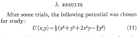
which translates to \(\alpha=1.0\), \(m=1\) and \(\omega=1\).
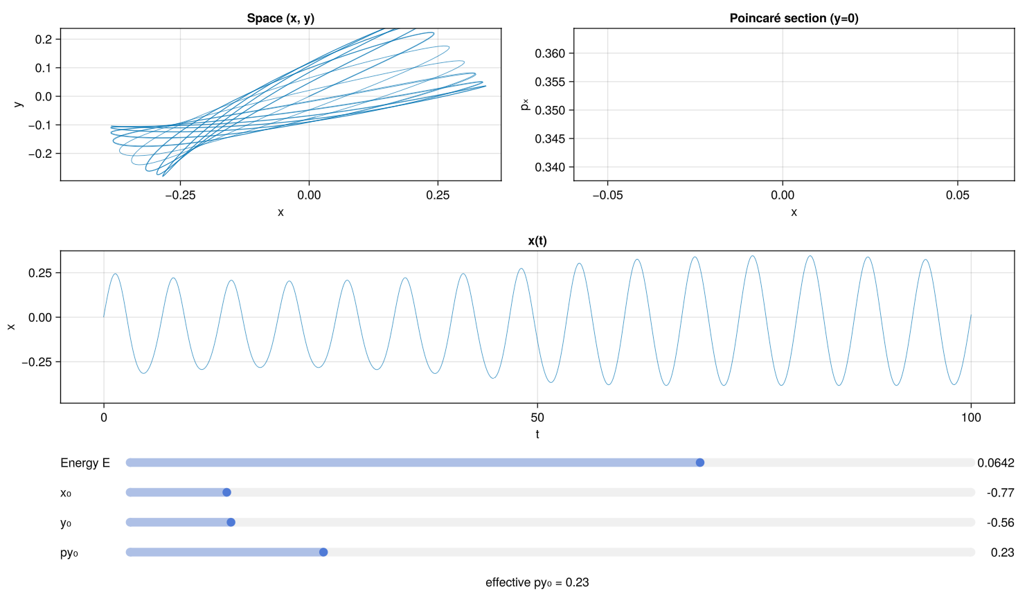
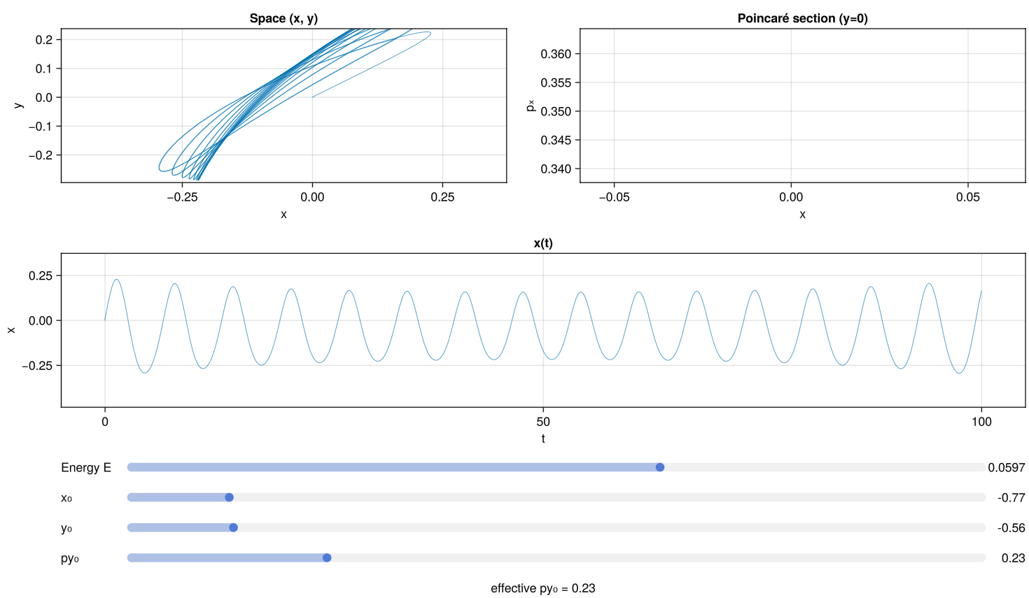
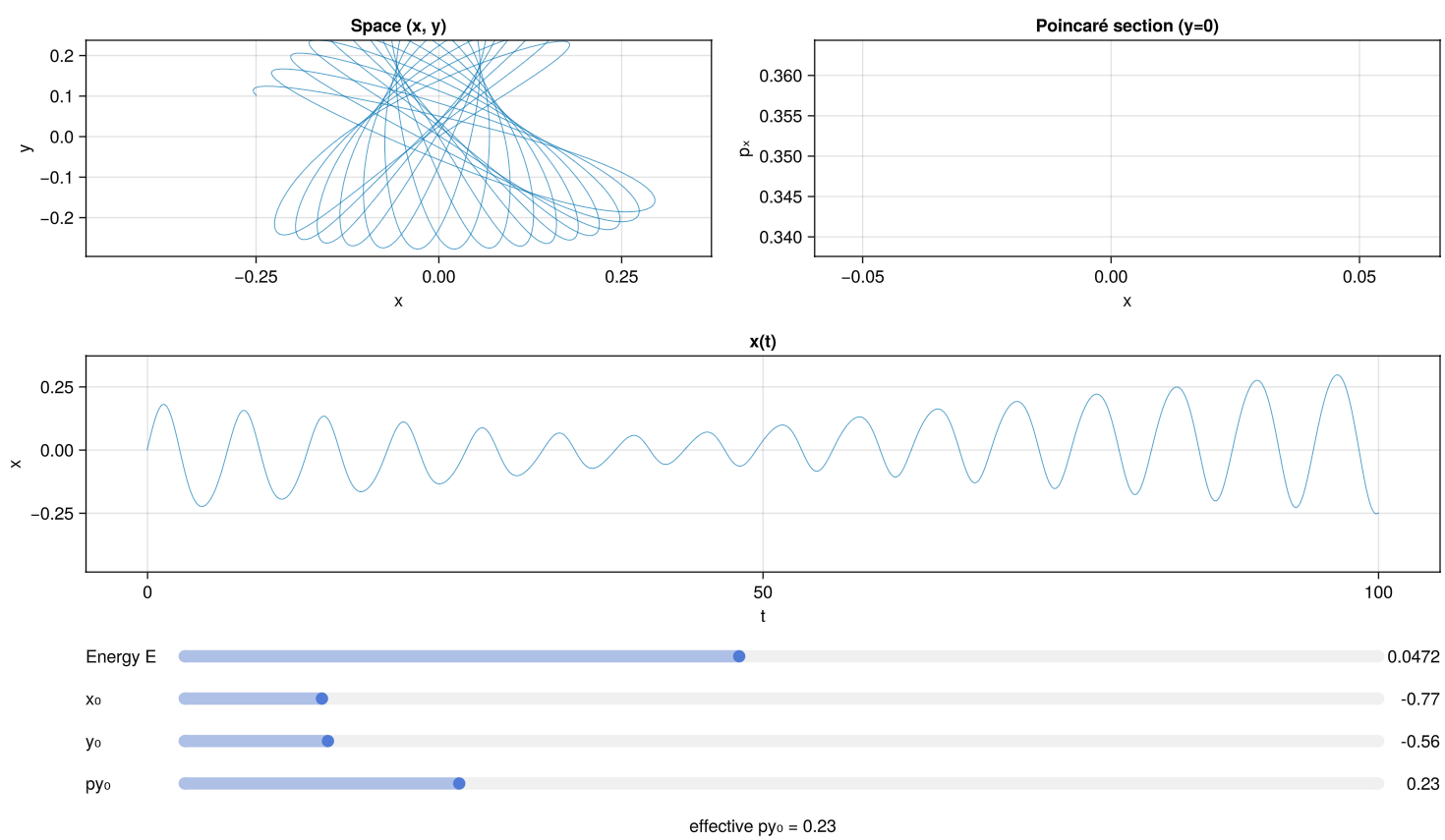
This results in the following plots depict the difference


The specific detail I obtain from this plot is, the initial-conditions-space that I need to sample.
- (\(x\), \(y\))–plane
- (\(p_x\), \(p_y\))–plane
- even distribution,
- weighted distribution based on regions of interest, i.e a “zoom”
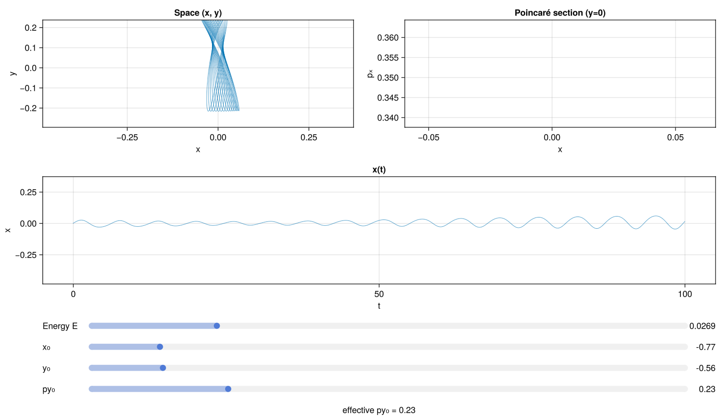
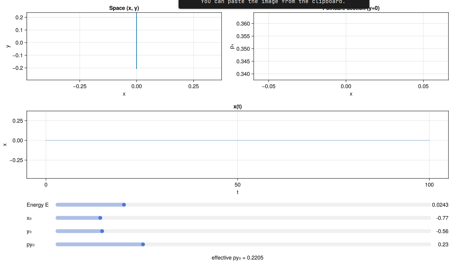
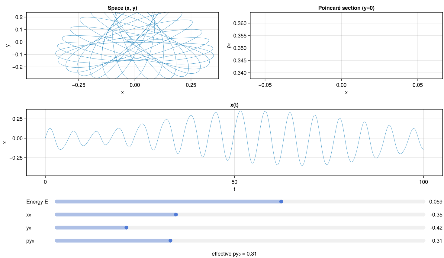
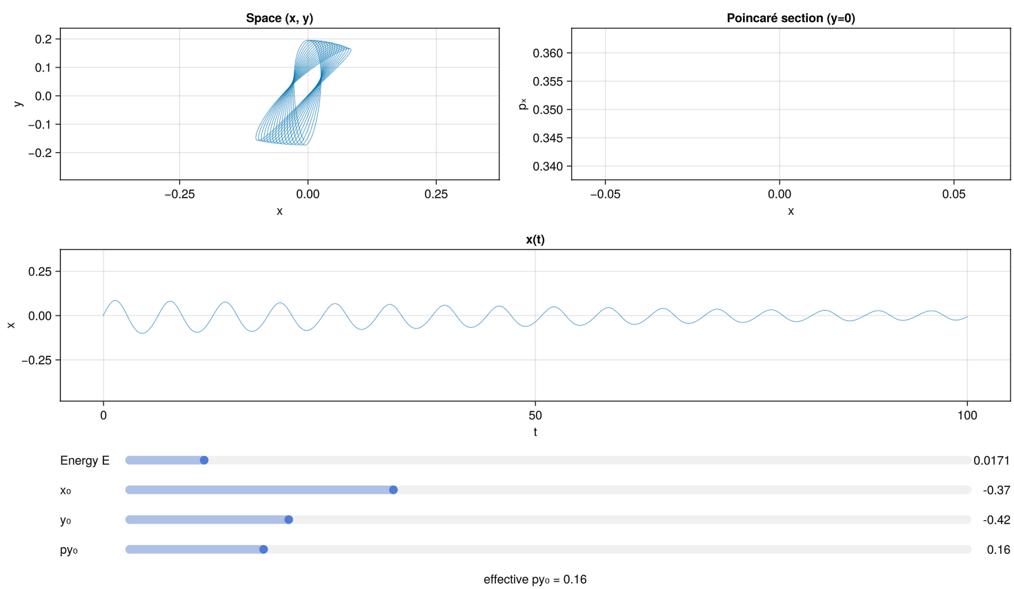
I have made the following observations running the following interesting observations of transitions, sudden changes on the kind of trajectories made in the x-y plane
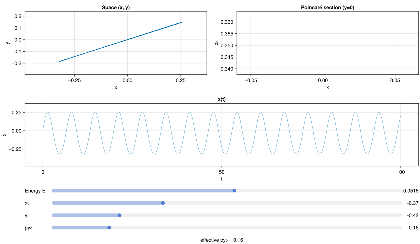
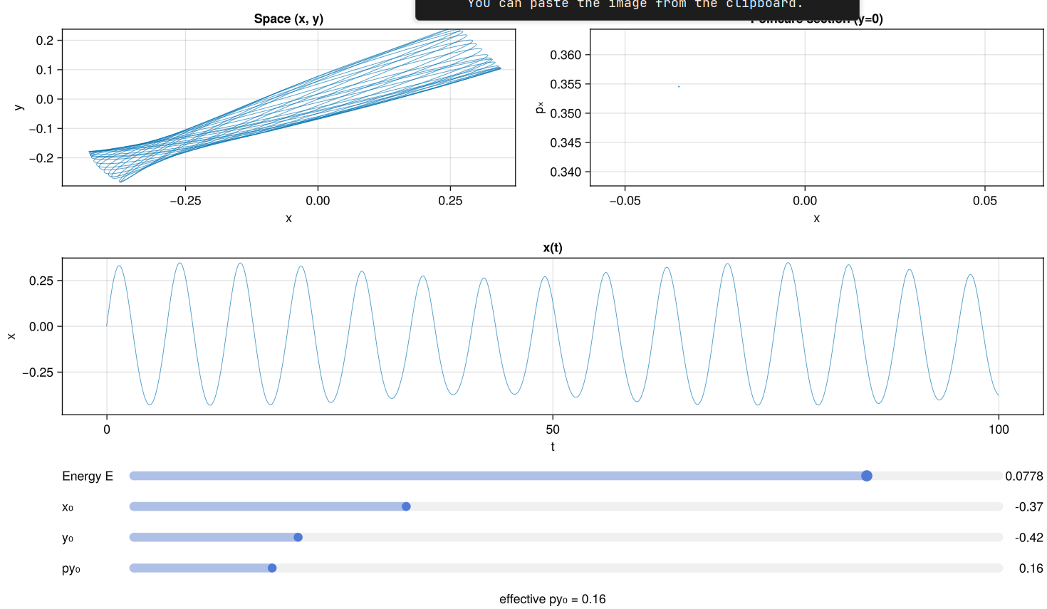
On implementation of Hénon-Heiles
Describing the error
- the issue arises for a parameter of \(\alpha=2\), where in contrast \(\alpha=1\) works fine.
- I am orientating myself on hénon-heiles paper (\(\alpha=2\), \(E=0.08333\))
- looking at the potential energy plot
potential energy

Parameters
| Parameter | Value | Units | Description |
|---|---|---|---|
| \(\alpha\) | 2.0 | — | Non-linear coupling strength |
| \(m\) | 1.0 | kg | Mass |
| \(\omega\) | 1.0 | 1/s | Harmonic oscillator frequency |
On implementation of Hénon-Heiles
These are two screen shots of the Hénon-Heiles potential
Parameters
| Parameter | Value | Units | Description |
|---|---|---|---|
| \(\alpha\) | 2.0 | — | Non-linear coupling strength |
| \(m\) | 1.0 | kg | Mass |
| \(\omega\) | 1.0 | 1/s | Harmonic oscillator frequency |
Lost Wonderers Thoughts:
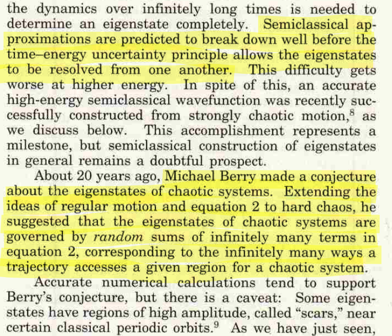
I spend an hour raading “Postmoden Quantummechanics” (Heller and Tomsovic 1993).
Semiclassical approximation of quantum amplitudes have a universal form and is given by \[\psi(x)=\sum_n \sqrt{P_n(x)} \,\exp\Big\{i \varphi_n(x)/\hbar\Big\},\] with
\(\varphi_n(x)\) – classical action along the \(n^\text{th}\) path reaching \(x\)
\(P_n(x)\) – classical probability
Implementation of Hénon-Heiles
So I have the Hamiltonian of the Hénon–Heiles potential
\[H(x,y,p_x,p_y)=\frac{(p_x^2+p_y^2)}{2m} + \frac{m\omega^2}{2}(x^2+y^2)+\alpha(x^2y-\frac{y^3}{3}).\]
We obtain the equations of motion by
\[\dot{q_i} =\frac{\partial H}{\partial p_i} \]
\[\dot{p_i} =-\frac{\partial H}{\partial q_i} \]
for canonical conjugate variables \((p_i,q_i)\) labeled by \(i\in\mathbb{N}\).
The resulting equation of motion in julia code:
function equations!(du, u, p, t)
    m, a, w = p
    x, y, px, py = u
    du[1] =  px
    du[2] =  py
    du[3] = -m*w^2*x - 2a*x*y
    du[4] = -m*w^2*y - a*(x^2 - y^2)
end
Here the potentials are defined:
potential(x, y; m=m, w=w, a=a) = m*w^2/2 *(x^2+y^2) + a*(x^2*y - y^3/3)

kinetic(px, py; m=m, w=w) = (px^2 + py^2)/(2*m)

hamiltonian(x, y, px, py; m=m, w=w, a=a) = kinetic(px, py, m=m, w=w) + potential(x,y, m=m, w=w, a=a)
And here the trajectory gets solved:
function solve_trajectory(u0; tspan=(0.0, 500.0), dt=0.1, p=param)
    prob = ODEProblem(equations!, u0, tspan, p)
    solve(prob, Vern9(), abstol=1e-10, reltol=1e-10, saveat=dt)
endTo do!
- [ ]
Lost Wonderers Thoughts:
Quantum Walk & Chaos
- Quantum Walk: linear equations, no chaos
- it has been used (Kamran et al. 2022) for encryption of pictures

To do!
yesterdays todo’s:*
checking in
I feel that I should read about implementing the Hénon & Heiles. I should also read their original paper.
Whilst working on Hénon & Heiles, I realize I need to get an in depth understanding of the Lagrange and Hamiltonian formalism!
Notes from Hénon & Heiles
Hénon and Heiles (1964) - on isolating and non isolating integrals A CLASSIFICATION OF THE INTEGRALS OF MOTION by George Contopoulos
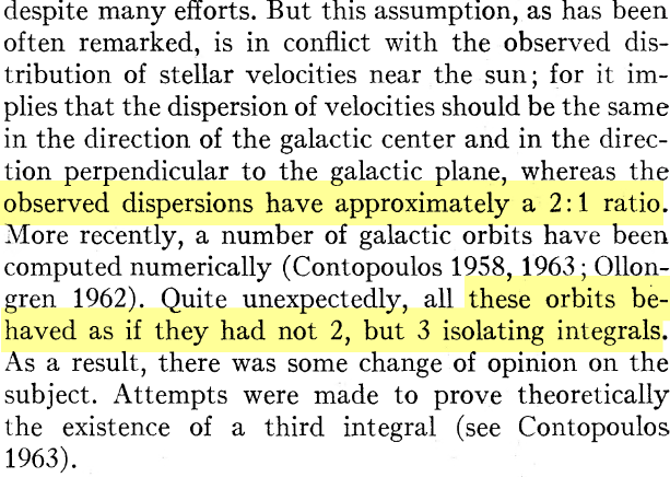
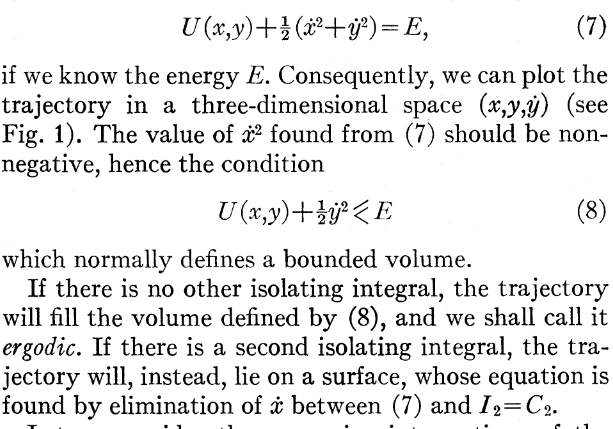
I did not understand much of section 2
a second read and note shed some light, here is an interesting paragraph describing what ergodic mean
a question they seem to be answering is how to find a proof of the existence of an non isolating integral
they speak of two integration schemes:
- Adams
- Runge-Kutta
Their analysis introduces terms as islands and chain of islands, dimension of islands, dense and need to be understood when I study this model
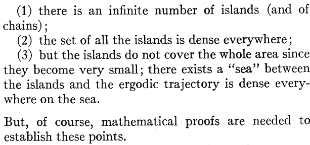
- “but the dimensions are so small that finding them is difficult” – is how the term dimensions gets used again
Yesterdays To do!
getting started: Hénon Heils Model
Comments for the day:
I first worked on some further workflow questions. Including a bash script for adding entries from the ‘glossary.json’ to the ‘glossary.qmd’ file and to the ’_quarto.qmd’ file, for latex macros or to initiate the day-log by the use of templates.
I use the ai-tool provided by claude to help generate the bash-scripts for workflow and to communicate about the structure of my workspace. I have general idea from previous projects how I want to structure my workspace - though I do not have the knowledge in coding in ‘bash’ or ‘yml’ etc…
So I use ai to set up my folder structure and to prepare the workflow. I also need to keep track of my ai usage for transparency.
suggested structure
- derivation
- considering derivation
- numerical implementation
observations
- original paper by Henon and Heiles Hénon and Heiles (1964)
- I came across, need to undertand: 6-D phase space -> 5 independant conservative integrals of the motion; seemingly, sure but I want a rigorous understanding
- results in 5 hyper surfaces, their intersections define the trajectories
- literature by Strogatz (2015) under chapter 12 strange attractors
- wikipedia
- ‘orbit diagram’ or ‘bifracation diagram’
- is the Héno Map the same as the Hénon–Heiles model? I dont think so!
Lost Wanders Thoughts:
- connections of strange attractor to Cantor Set (Arnold1989?) p. 430-431;
- gets me to think about how ternary number representation (base 3) is a useful way to analyze the Cantor set
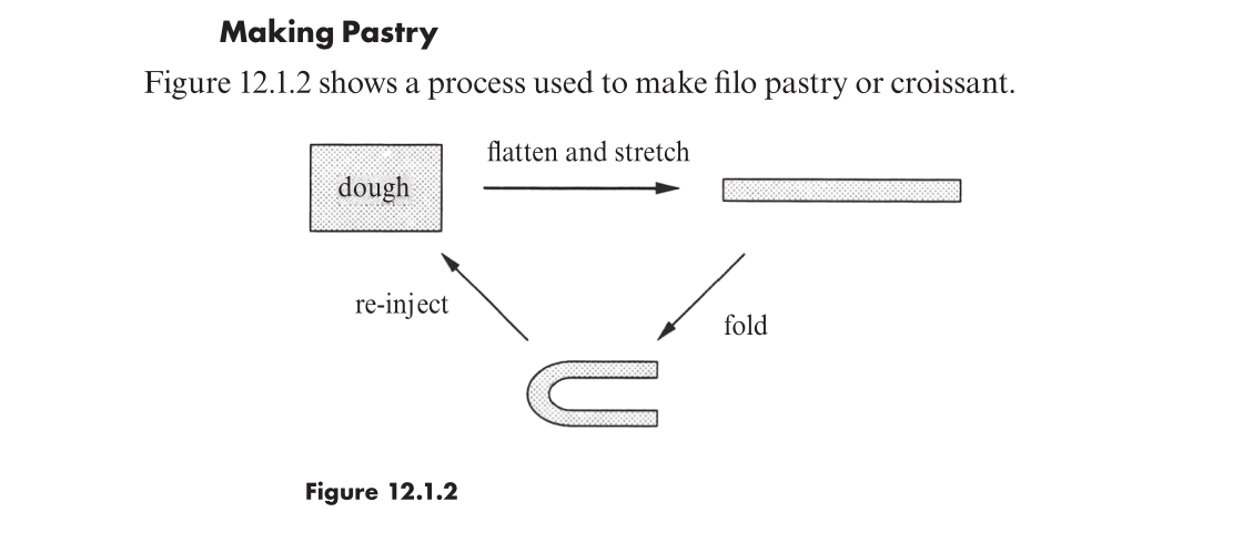
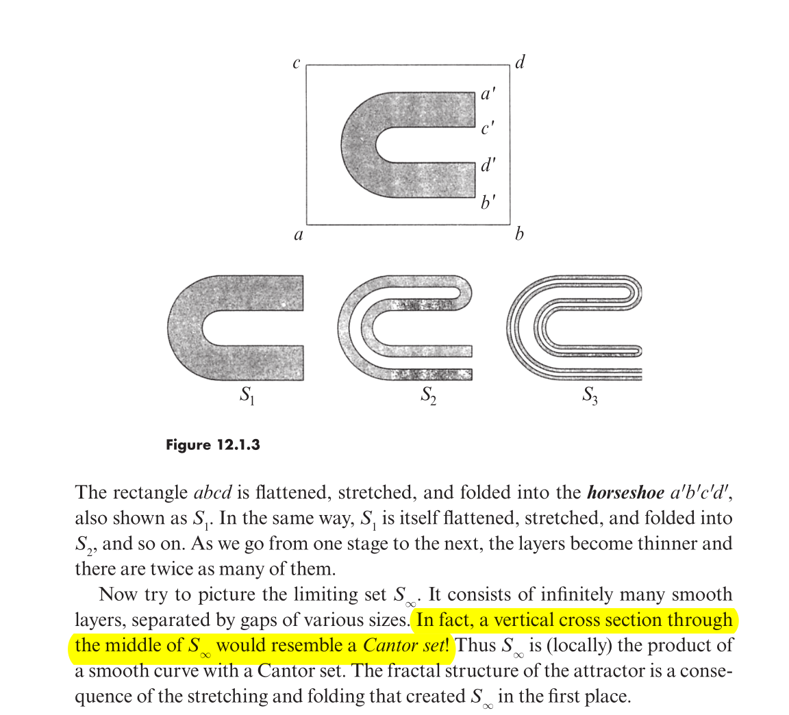
…
To do!
Interests:
- universality -> quantum chaos A Field Theory Approach to Universality in Quantum Chaos
- random matrix theory?
- phase transitions as models for non-linear systems
- how non-linear systems develop as a function of degrees of freedom
Issues:
- low understanding of basic concepts
- I want to learn by doing, so that I come across basic concepts and problems
- how to find a model to start?
talk with Benoit:
- Hénon Heilses Hamiltonian -> classical chaos (connection to Toda potential, integrable)
\[V(x,y)=1/2(x^2+y^2)+x^2y - 1/3 y^3\]
- Heno Heiles model, by Toda potential -> 3D; resulting in Heno Heiles 3D?
- obtaining higher order DOF by taking integral system, pert
- find the models in the books
- computational methods (pioncare cross section)